Log-Likelihood

Because small values are very unstable in computers, we use the Log-Likelihood. It uses a sum and applies the logarithm to every datapoint.

L(θ)=∏i=1Np(si∣θ)=∗∑i=1Nlog⁡[p(si∣θ)]=ℓ(θ)\begin{equation} \boldsymbol{L}(\boldsymbol{\theta})=\prod_{i=1}^{N} p\left(\mathbf{s}_{i} \mid \boldsymbol{\theta}\right) \stackrel{*}{=} \sum_{i=1}^{N} \log \left[p\left(\mathbf{s}_{i} \mid \boldsymbol{\theta}\right)\right]=\boldsymbol{\ell}(\boldsymbol{\theta}) \end{equation}

Rewrite Log-Likelihood by inserting the Logistic Function and applying the logarithm to the sum

L(θ)=log⁡(∏i=1mP(yi∣xi))=∑i=1mlog⁡(g(θ⊤xi)yi(1−g(θ⊤xi))1−xi)\begin{aligned} &\mathscr{L}(\theta)=\log \left(\prod_{i=1}^m P\left(y_i \mid x_i\right)\right) \\ &=\sum_{i=1}^m \log \left(g\left(\theta^{\top} x_i\right)^{y_i}\left(1-g\left(\theta^{\top} x_i\right)\right)^{1-x_i}\right) \end{aligned}

then again applying the logarithm to the exponents

=∑i=1myilog⁡(g(θ⊤xi))+(1−yi)log⁡(1−g(θ⊤xi))=\sum_{i=1}^m y_i \log \left(g\left(\theta^{\top} x_i\right)\right)+\left(1-y_i\right) \log \left(1-g\left(\theta^{\top} x_i\right)\right)

then using the definition of the Logistic Function to get

=∑i=1myilog⁡(eθ⊤xi1+eθ⊤xi)+(1−yi)log⁡(11+eθ⊤xi)=∑i=1myiθ⊤xi+log⁡11+eθ⊤xi\begin{aligned} &=\sum_{i=1}^m y_i \log \left(\frac{e^{\theta^{\top} x_i}}{1+e^{\theta^{\top} x_i}}\right)+\left(1-y_i\right) \log \left(\frac{1}{1+e^{\theta^{\top} x_i}}\right) \\ &=\sum_{i=1}^m y_i \theta^{\top} x_i+\log \frac{1}{1+e^{\theta^{\top} x_i}} \end{aligned}

and finally using the definition again to get

=∑i=1myiθ⊤xi+log⁡(1−g(θ⊤xi))=\sum_{i=1}^m y_i \theta^{\top} x_i+\log \left(1-g\left(\theta^{\top} x_i\right)\right)

We can use this much simpler form of the equation to calculate the Gradient of the Log-Likelihood:

∇θL(θ)=∇θ(∑i=1myiθ⊤xi+log⁡(1−g(θ⊤xi)))=∑i=1myixij+11−g(θ⊤xi)(−g(θ⊤xi)(1−g(θ⊤xi))xij=∑i=1myixij−g(θ⊤xi)xij=∑i=1m(yi−g(θ⊤xi)xij\begin{aligned} &\nabla_\theta \mathcal{L}(\theta)=\nabla_\theta\left(\sum_{i=1}^m y_i \theta^{\top} x_i+\log \left(1-g\left(\theta^{\top} x_i\right)\right)\right) \\ &=\sum_{i=1}^m y_i x_{i j}+\frac{1}{1-g\left(\theta^{\top} x_i\right)}\left(-g\left(\theta^{\top} x_i\right)\left(1-g\left(\theta^{\top} x_i\right)\right) x_{i j}\right. \\ &=\sum_{i=1}^m y_i x_{i j}-g\left(\theta^{\top} x_i\right) x_{i j}=\sum_{i=1}^m\left(y_i-g\left(\theta^{\top} x_i\right) x_{i j}\right. \end{aligned}

and the Hessian Matrix like this

∇θ∇θL(θ)=∇θ∑i=1m(yi−g(θ⊤xi)xij=∑i=1m−g(θ⊤xi)(1−g(θ⊤xi))xixi⊤\begin{aligned} &\nabla_\theta \nabla_\theta \mathcal{L}(\theta)=\nabla_\theta \sum_{i=1}^m\left(y_i-g\left(\theta^{\top} x_i\right) x_{i j}\right. \\ &=\sum_{i=1}^m-g\left(\theta^{\top} x_i\right)\left(1-g\left(\theta^{\top} x_i\right)\right) x_i x_i^{\top} \end{aligned}

We can now use the Newton Method to iteratively calculate the best parameters:

θk+1=θk−(∂2∂θ∂θTL(θk))−1∂∂θL(θk)\theta^{k+1}=\theta^k-\left(\frac{\partial^2}{\partial \theta \partial \theta^T} \mathcal{L}\left(\theta^k\right)\right)^{-1} \frac{\partial}{\partial \theta} \mathcal{L}\left(\theta^k\right)

For Gaussian

We then insert the Gaussian Distribution of yy like this:

∑i=1Nlog⁡[p(si∣θ)]=∑i=1Nlog⁡[(12πσ2)12e−12σ2(yi−wTxi)2]=−12σ2∑i=1N(yi−wTxi)2−N2log⁡(2πσ2)\begin{equation} \begin{aligned} \sum_{i=1}^{N} \log \left[p\left(\mathbf{s}_{i} \mid \boldsymbol{\theta}\right)\right] &=\sum_{i=1}^{N} \log \left[\left(\frac{1}{2 \pi \sigma^{2}}\right)^{\frac{1}{2}} e^{-\frac{1}{2 \sigma^{2}}\left(\mathbf{y}_{i}-\mathbf{w}^{\mathrm{T}} \mathbf{x}_{i}\right)^{2}}\right] \\ &=-\frac{1}{2 \sigma^{2}} \sum_{i=1}^{N}\left(\mathbf{y}_{i}-\mathbf{w}^{\mathrm{T}} \mathbf{x}_{i}\right)^{2}-\frac{N}{2} \log \left(2 \pi \sigma^{2}\right) \end{aligned} \end{equation}

The Log-Likelihood can then be simplified to a negative constant times the ==Residual Sum of Squares (Also called the Loss)== and adding another constant at the back.
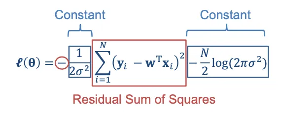
IMG - Loss?.png

We now have a minus sign in the front. That is why we have to minimize the Residual Sum of Squares to maximize the Log-Likelihood.

The Loss is convex thus it has a unique minimum which can be calculated with: